Decoding the 2025 Presidential Address: Text Mining and Data Visualizations

The 2025 Presidential Address has concluded, and as always, it’s left us with a lot to unpack. Beyond the immediate reactions and soundbites, a deeper dive into the address’s content can reveal hidden patterns and insights. In this post, we’ll explore how text mining and data visualizations can help us understand the key themes and nuances of the speech.

The Power of Text Mining

Text mining, also known as text analytics, allows us to extract meaningful information from unstructured text data. In the context of the Presidential Address, this means we can:

• Identify Key Topics: By analyzing the frequency of words and phrases, we can pinpoint the most prominent themes discussed by the president.
• Sentiment Analysis: We can gauge the overall tone of the speech, whether it’s optimistic, cautious, or critical, by analyzing the emotional connotations of the words used.
• Topic Modeling: Algorithms can group related words and phrases into distinct topics, providing a structured overview of the speech’s content.
• Keyword Extraction: We can automatically identify the most important keywords and phrases, highlighting the core message of the address.

Visualizing the Data

In tihs case the data are words. Clearly, one type of visualization is just reading the text, but let’s try to do something that require less effort for the reader. Here are some visualization techniques that can be applied:

• Word Clouds: These visually striking representations display the most frequent words in the speech, with larger words indicating higher frequency. This provides a quick overview of the key topics.
• Bar Charts: These can be used to compare the frequency of different topics or keywords, allowing for easy comparison.
• Line Graphs: These can illustrate the sentiment over the course of the speech, showing how the president’s tone changed throughout the address.

Let’s apply these methods to President Trumps address to Congress

First, we need that acutal text data. You can find the transcript on many websites, but here is one

Copy and paste the transcript to the a text file. We will need this file to bring in the text data into R. My file is called trump.txt.

We will use a couple of text mining packages: tm,wordcloud,SnowballC, tidytext, tidyverse, and sentimentr.

R code for Word Frequencies

# Install required packages
install.packages(c("tm", "wordcloud","SnowballC","tidytext","tidyverse","sentimentr"))

# Load libraries
library(tm)
library(wordcloud)
library(SnowballC)
library(tidytext)
library(tidyverse)
library(sentimentr)

# Create a corpus variable
# readlines command reads in the text file into R
trump <- readLines("~/Downloads/trump.txt", encoding = "UTF-8")
trump_text <- paste(trump, collapse = " ") # Combine lines into a single text

# Most of the data manipulation requires that our text is in a data.frame format.
trump_tribble <- tibble(text=trump_text)
trump_df <-trump_tribble %>%
  unnest_tokens(word, text)

# It is generally a good idea to remove stopwords. These are commonly used words like "a", "the", and "and"
clean_speech_df <- trump_tribble %>%
  unnest_tokens(word, text) %>%
  anti_join(stop_words, by = "word")

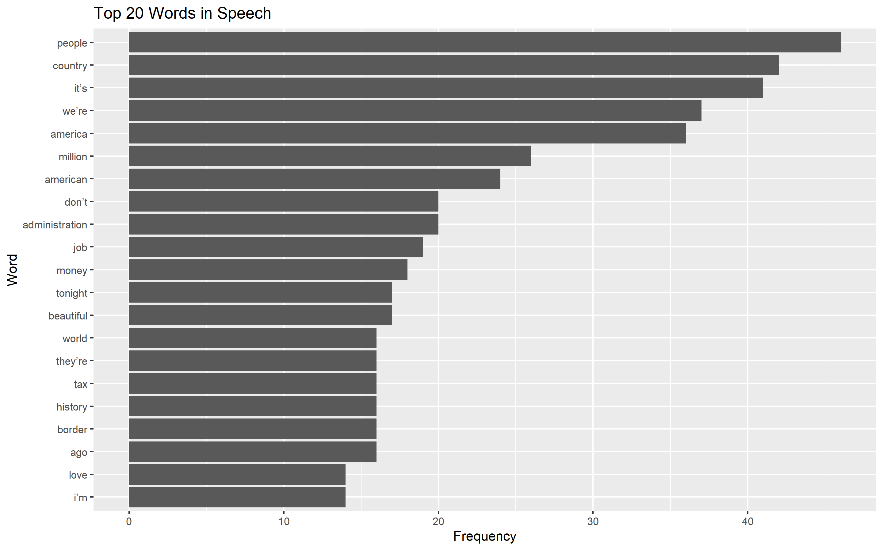
# Creates a bar graph of the top 20 words used
word_counts <- clean_speech_df %>%
  count(word, sort = TRUE)
word_counts %>%
  top_n(20) %>%
  ggplot(aes(x = reorder(word, n), y = n)) +
  geom_col() +
  coord_flip() +
  labs(title = "Top 20 Words in Speech", x = "Word", y = "Frequency")

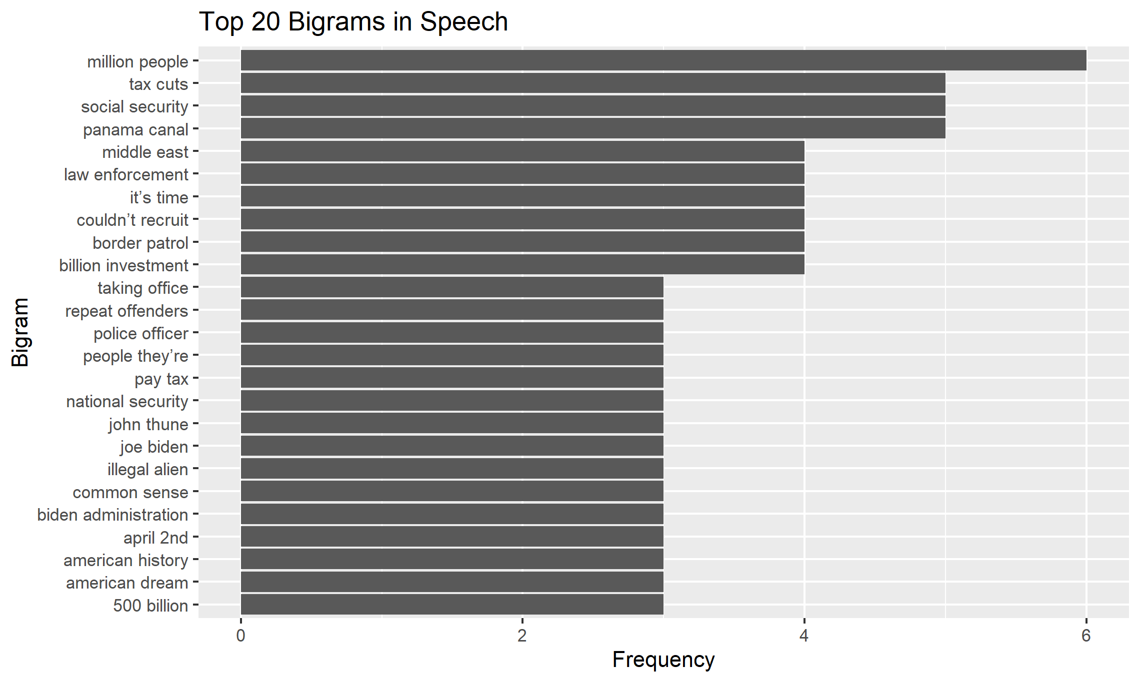
# Tokenize into bigrams
bigram_counts <- trump_tribble %>%
  unnest_tokens(bigram, text, token = "ngrams", n = 2) %>%
  separate(bigram, into = c("word1", "word2"), sep = " ") %>%  # Split bigrams into two words
  filter(!word1 %in% stop_words$word, !word2 %in% stop_words$word) %>%  # Remove stopwords
  unite(bigram, word1, word2, sep = " ") %>%  # Reunite words into bigrams
  count(bigram, sort = TRUE)  # Count bigram frequency

# Creates a bar graph for bigrams
bigram_counts %>%
  top_n(20) %>%
  ggplot(aes(x = reorder(bigram, n), y = n)) +
  geom_col() +
  coord_flip() +
  labs(title = "Top 20 Bigrams in Speech", x = "Bigram", y = "Frequency")

In the code above we do several things.

• Bring the data into R
• Tokenized words so it is easier for R to handle.
• Clean the data by removing stopwords. The library Snowball contains a list of stopwords like “I”, “and”, “the” etc. You can find the whole list here.
• Now we can start processing these words by making barcharts of the most frequently used words.

Below I show the most commonly used single words and bigram (two word combinations) used in the speech.

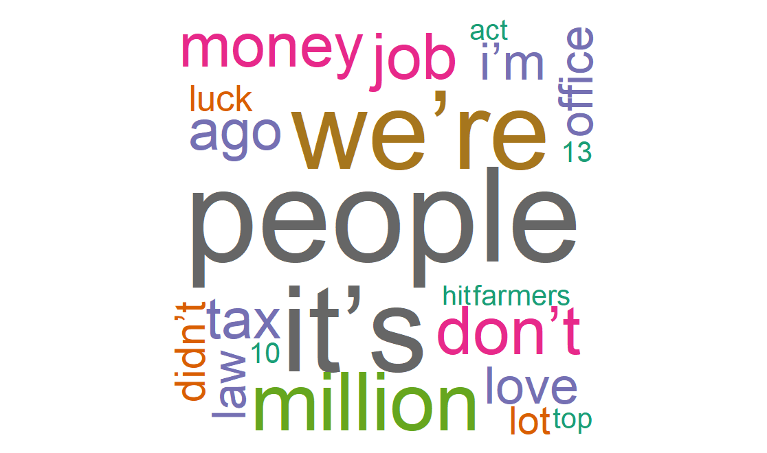
Wordcloud

We can also take the data and make a wordcloud.

# Wordcloud
set.seed(123) # For reproducibility
wordcloud(words = word_counts$word, freq = word_counts$n, min.freq = 1,
          max.words = 200, random.order = FALSE, rot.per = 0.35,
          colors = brewer.pal(8, "Dark2"))

Sentimental Analysis

Lastly, we can use sentimental analysis, which tells you how positive or negative a certain word is, to analyze the speech.

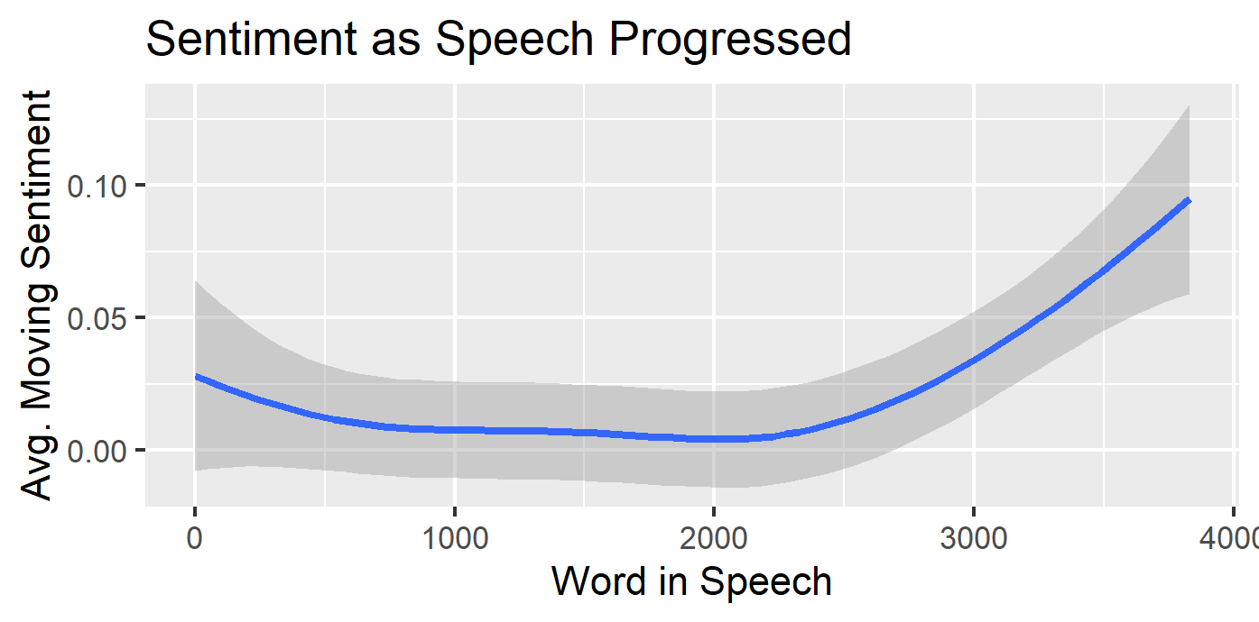
I will take the sentiment score of each word in order of the speech, then use a smooth mean so that we can see how the sentiment progress through the speech.

# Sentimental Anlaysis
trump_words<-unlist(clean_speech_df) # untokenizes the word list
trump_sent<-sentimentr::sentiment(trump_words) # provides the sentimental scores
# Next we graph the sentimental scores.
ggplot(trump_sent,aes(x=element_id, y=sentiment))
  +geom_smooth()+xlab("Word in Speech")+ylab("Avg. Moving Sentiment")
  +labs(title = "Sentiment as Speech Progressed")

As you would expect the speech starts “mid” as the kids would say, but then builds some steam and becomes more positive towards the end.