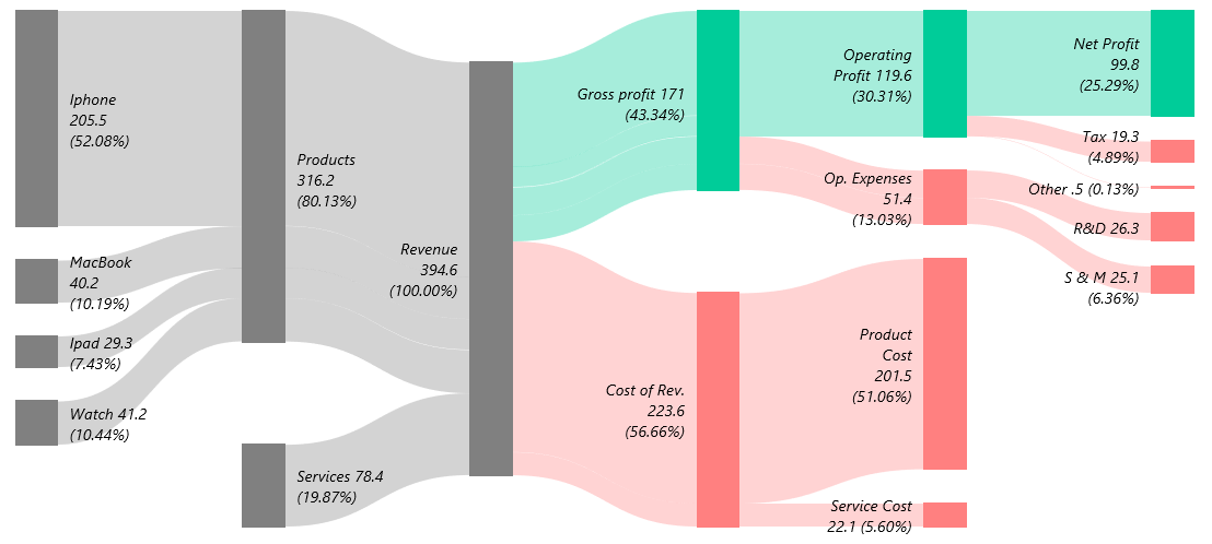
In this blog post we are going to take data from IPUMS and create a Sankey Chart. Data visualization is a growing part of business reports and data journalism. On way to demonstrate how flows move from one category to another is through the use of Sankey plots.

In today’s exercise, I used the 2023 American Community Survey (ACS) to look at which occupations Econ majors enter. The ACS has separate college major and occupation codes. I obtain the data using the online tool in IPUMS. You will need to create your own account if you wish to replicate this exercise.

I have provided a short video explainer on youtube

IPUMS is a US Census base dataset. You can use the online tool do most of the work here. Select the ACS as your data source

You can download the data, which I use with the code below here.

The variables we will need are degree field detail (degfieldd) and occupation code (occ)

Degfieldd will be your column variable and OCC will be your row variable.

In degfieldd we do not need all of the degrees just a few. 6205 = Business Economics and 5501 = Economics I put this in the filter option so that we only have econ majors. degfield(r: 5501 “Economics”; 6205 “Business Economics”)

Enter occ in the row field and sex in the column field

Then select run table.

Download the data but keep only the top 20 jobs. Or aggregate them by industry as I did in the video.

If you get it to work with just economics and the top 20 jobs, then try doing it will all of the majors with the code below.

degfieldd(r: 5501 “Economics” ; 6205 “Business Economics”; 6206 “Marketing”; 6207 “Finance”; 6212 “CIS”; 6201 “Accounting”; 6203 “Management”)

If you don’t want to use R then try this website hat tip to Andrew Friedson https://sankeymatic.com/

# Library
library(networkD3)
library(dplyr)

# Enter data here. Source is your first column, Target is your second column

# From these flows we need to create a node data frame: it lists every entities involved in the flow
nodes <- data.frame(
  name=c(as.character(econocc$Source), 
         as.character(econocc$Target)) %>% unique()
)

# With networkD3, connection must be provided using id, not using real name like in the links dataframe.. So we need to reformat it.
econocc$IDsource <- match(econocc$Source, nodes$name)-1 
econocc$IDtarget <- match(econocc$Target, nodes$name)-1

# Make the Network
p <- sankeyNetwork(Links = econocc, Nodes = nodes,
                   Source = "IDsource", Target = "IDtarget",
                   Value = "Amount", NodeID = "name", 
                   sinksRight=FALSE, fontSize = 14)
p

# you save it as an html
saveNetwork(p, "p.html")

library(webshot)
# you convert it as png
webshot("p.html","sn.png", vwidth = 1200, vheight = 500)

Here is a link to the end result